Gibbs sampling

• Abstract
• What is Gibbs sampling?
• How does it work?
  • Procedure
  • Example
• Why does it work?
  • Markov Chain Monte Carlo (MCMC)
  • Proof

Abstract

This article provides the recipes, simple Python codes and mathematical proof to the most basic form of Gibbs sampling.

What is Gibbs sampling?

Gibbs sampling is a method to generate samples from a multivariant distribution $P(x_1,x_2,\dots ,x_d)$ using only conditional distributions $P(x_1|x_2\dots x_d)$, $P(x_2|x_1,x_3\dots x_d)$ and so on. It is used when the original distribution is hard to calculate but the conditional distributions are available.

How does it work?

Procedure

Starting with a sample $\mathbf{x}=(x_1,x_2\dots x_d)$, to generate a new sample $\mathbf{y}=(y_1,y_2\dots y_d)$, do the following

1. Sample $y_1$ from $P(y_1|x_2,x_3\dots x_d)$.
2. Sample $y_2$ from $P(y_2|y_1,x_3\dots x_d)$.
3. Sample $y_3$ from $P(y_3|y_1,y_2,x_4\dots x_d)$
4. … and so on. The last term is sampling $y_d$ from $P(y_d|y_1,y_2\dots y_{d-1})$.
5. Now we have the new sample $\mathbf{y}$. Repeat for the next sample.

Note that the value of a new sample depends only on the the previous one, and not the one before, Gibbs sampling belongs to a class of methods called Markov Chain Monte Carlo (MCMC).

Example

Consider a mixture of two 2-dimensional normal distribution below with joint distribution $P(x,y)=\frac{1}{2}(\mathcal{N}({\mu }_1,{\text{cov}}_1)+\mathcal{N}({\mu }_2,{\text{cov}}_2))$.

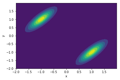
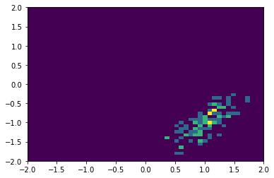
We can use the procedure above to to generate samples using only the conditional distribution $P(x|y)$ and $P(y|x)$. The sample chain could initially be trapped in one local distribution:

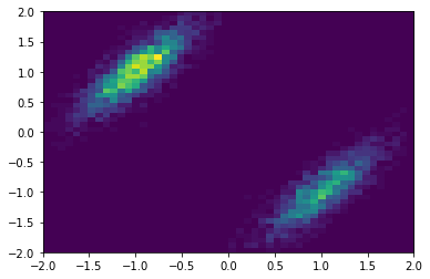
But if enough number of points are sampled, the original distribution is recovered:

The codes that generate this example can be found here.

Why does it work?

This section outlines the proof of Gibbs sampling. I mostly follow MIT 14.384 Time Series Analysis, Lectures 25 and 26.

Markov Chain Monte Carlo (MCMC)

Gibbs sampling generates a Markov chain. That’s obvious because the series $X^{(1)}$, $X^{(2)}$, $X^{(3)}$ … depends only on the previous value. An important concept to understand is the transition Probability $P(\mathbf{x},\mathbf{y})$, the probability of generating sample $\mathbf{y}$ from the previous sample $\mathbf{x}$.

Suppose we want to sample a distribution $\pi (\mathbf{x})$, we want to generate samples in a way that the new sample still follows distribution $\pi (\mathbf{x})$. Mathematically, for transition probability $P(\mathbf{x},\mathbf{y})$, the probability measure $\pi (\mathbf{x})$ is invariant if

$$\begin{array}{}\text{(1)}& \pi (\mathbf{y})=\int P(\mathbf{x},\mathbf{y})\pi (\mathbf{x})d\mathbf{x}\end{array}$$

and the transition probability is

1. irreducible (i.e. any point can reach any other points)
2. aperiodic

The MCMC problem is to find a transition probability $P(\mathbf{x},\mathbf{y})$ such that $\pi (\mathbf{x})$ is invariant.

Proof

The procedure of Gibbs sampling outlined previously can be written as a transition probability

$$\begin{array}{}\text{(2)}& P(\mathbf{x},\mathbf{y})& =\pi (y_1|x_2,x_3,..,x_d)\pi (y_2|y_1,x_3,..,x_d)...\pi (y_d|y_1,y_2,..,y_{d-1})\text{(3)}& & =\prod _k\pi (y_k|y_1...y_{k-1},x_{k+1}...x_d)\end{array}$$

Let $\pi (\mathbf{x})$ be the distribution we want to sample from. We need to show $\pi (\mathbf{x})$ is invariant under this transition, i.e.

$$\begin{array}{}\text{(4)}& \int P(\mathbf{x}\mathbf{,}\mathbf{y})\pi (\mathbf{x})d\mathbf{x}=\pi (\mathbf{y})\end{array}$$

In other words, if we follow $P(\mathbf{x},\mathbf{y})$ to get new sample $\mathbf{y}$ based on the previous sample $\mathbf{x}$, and repeat this process over and over again, we stay in the same distribution $\pi (\mathbf{x})$.

Since we need to integrate over $\mathbf{x}$, the first thing is to rewrite $P(\mathbf{x},\mathbf{y})$ using Bayes rule so that there’s no conditional on $\mathbf{x}$. Bayes rule is

$$P(A|B)P(B)=P(B|A)P(A)$$

or if there’s always a conditional on $C$:

$$P(A|B,C)P(B|C)=P(B|A,C)P(A|C)$$

Using

$$\begin{array}{}\text{(5)}& A& =y_k\text{(6)}& B& =x_{k+1},...,x_d\text{(7)}& C& =y_1,..,y_{k-1}\end{array}$$

We get

$$\begin{array}{}\text{(8)}& \pi (y_k|y_1...y_{k-1},x_{k+1}...x_d)=\frac{\pi (x_{k+1},...,x_d|y_1,..,y_k)\pi (y_k|y_1,..,y_{k-1})}{\pi (x_{k+1},...,x_d|y_1,..,y_{k-1})}\end{array}$$

Substituting this to Eq.($\text{4}$), and noticing that $\pi (y_k|y_1,..,y_{k-1})$ does not depend on the integrating variable $\mathbf{x}$,

$$\begin{array}{}\text{(9)}& \int P(\mathbf{x}\mathbf{,}\mathbf{y})\pi (\mathbf{x})d\mathbf{x}=\prod _k\pi (y_k|y_1,..,y_{k-1})\int \prod _k\frac{\pi (x_{k+1},...,x_d|y_1,..,y_k)}{\pi (x_{k+1},...,x_d|y_1,..,y_{k-1})}\pi (\mathbf{x})d\mathbf{x}\end{array}$$

The first product

$$\begin{array}{}\text{(10)}& \prod _k\pi (y_k|y_1,..,y_{k-1})=\pi (\mathbf{y})\end{array}$$

because

$$\begin{array}{}\text{(11)}& \pi (\mathbf{y})& =\pi (y_1,y_2,..,y_d)\text{(12)}& & =\pi (y_d|y_1,..,y_{d-1})\pi (y_1,..,y_{d-1})\text{(13)}& & =\pi (y_d|y_1,..,y_{d-1})\pi (y_{d-1}|y_1,..,y_{d-2})\pi (y_1,..,y_{d-2})\text{(14)}& & \text{... and so on}\end{array}$$

So we have

$$\begin{array}{}\text{(15)}& \int P(\mathbf{x}\mathbf{,}\mathbf{y})\pi (\mathbf{x})d\mathbf{x}=\pi (\mathbf{y})\int \prod _k\frac{\pi (x_{k+1},...,x_d|y_1,..,y_k)}{\pi (x_{k+1},...,x_d|y_1,..,y_{k-1})}\pi (\mathbf{x})d\mathbf{x}\end{array}$$

We need to show the integral on the right hand side to be exactly 1.

We start by writing out the terms explicitly and use $\pi (x_1,..x_d)=\pi (x_1|x_2\dots x_d)\pi (x_2\dots x_d)$,

$$\begin{array}{}\text{(16)}& \int \prod _k\frac{\pi (x_{k+1},...,x_d|y_1,..,y_k)}{\pi (x_{k+1},...,x_d|y_1,..,y_{k-1})}\pi (\mathbf{x})d\mathbf{x}=\int \frac{\pi (x_2...x_d|y_1)}{\cancel{\pi (x_2...x_d)}}\frac{\pi (x_3...x_d|y_1,y_2)}{\pi (x_3...x_d|y_1)}...\pi (x_1|x_2...x_d)\cancel{\pi (x_2...x_d)}d{x}_{1}d{x}_2...d{x}_d\end{array}$$

The only term that depends on $x_1$ is $\pi (x_1|x_2\dots x_d)$ and it is integrated out to be 1. The integral becomes

$$\begin{array}{}\text{(17)}& =\int \frac{\pi (x_2...x_d|y_1)}{\pi (x_3...x_d|y_1)}\frac{\pi (x_3...x_d|y_1,y_2)}{\pi (x_4...x_d|y_1,y_2)}...\pi (x_d|y_1...y_{d-1})d{x}_2...d{x}_d\end{array}$$

Turning each fraction into a conditional probability

$$\begin{array}{}\text{(18)}& \frac{\pi (x_2...x_d|y_1)}{\pi (x_3...x_d|y_1)}=\pi (x_2|x_3..x_d,y_1)\end{array}$$

and so on. The integral becomes

$$\begin{array}{}\text{(19)}& =\int \pi (x_2|x_3..x_d,y_1)\pi (x_3|x_4..x_d,y_1,y_2)...\pi (x_d|y_1...y_{d-1})d{x}_2...d{x}_d\end{array}$$

Only the first term depends on $x_2$ and it is integrated out to be 1. After that, only the leading term depends on $x_3$ and it is integrated out to be 1 and so on. Therefore the whole integral is 1 resulting in

$$\begin{array}{}\text{(20)}& \int P(\mathbf{x}\mathbf{,}\mathbf{y})\pi (\mathbf{x})d\mathbf{x}=\pi (\mathbf{y})\end{array}$$

So the transition probability from Gibbs sampling is invariant. If we sample according to the Gibbs scheme, we can get unbiased samples of $\pi (\mathbf{x})$.