Deep dive into variational auto-encoder (Part 2)
An in-depth notes on VAE. Part 2 covers pytorch implementation.
In this article, I will go through implementing variational autoencoder step-by-step. The following code is tested on pytorch 1.4. Jupyter notebook can be found here.
One of the most powerful application of auto-encoder is that it can generate gradual changes through interpolation of latten variables. For example, we can produce “intermediate digits between 1 and 4:

This article will cover:
Code implementation
Model definition
First we define the parameters to be used in the model.
import torchvision
import torch
import matplotlib.pyplot as plt
from torch import nn
import numpy as np
import torch.nn.functional as F
import time

use_gpu = True  # use GPU or not
latent_size = 48  # dimension of latent variable. Should be much smaller than the image size
learning_rate = 0.001
train_batch_size = 128   # size of traning batch
data_dir = '/tmp'
data_size = 28*28 # size of mnist image
encoder_hidden_size = latent_size*2
decoder_hidden_size = latent_size*2
max_epochs = 10
opt = 'adam'  # adam or rms
Next, load the training dataset. Torchvision provides an interface that can conveniently load the MNIST data. They are 28 x 28 pixel grey scale images. We will later convert them to black-and-white images for simplicity.
train_data = torch.utils.data.DataLoader(
torchvision.datasets.MNIST(data_dir, train=True, download=True,
                         transform=torchvision.transforms.Compose([
                           torchvision.transforms.ToTensor(),
                           torchvision.transforms.Normalize(
                             (0.1307,), (0.3081,))
                         ])),
                        batch_size=train_batch_size, shuffle=True)
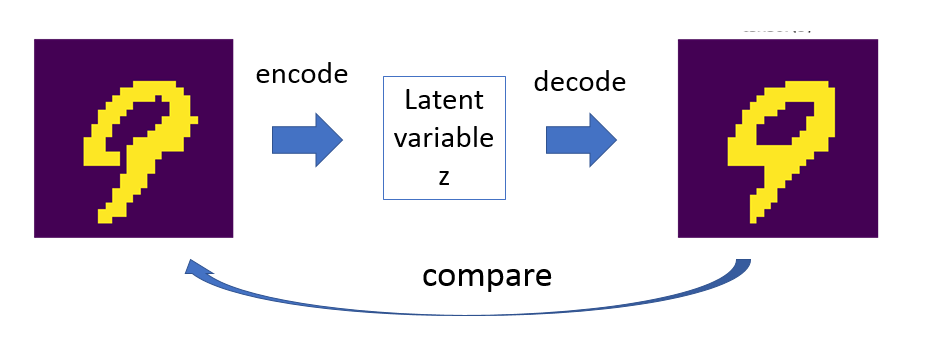
We then define the encoder and decoder models. The encoder coverts the digit image latent variable $z$. The decoder goes the other way, i.e. converting $z$ back to image and compare how well we get back the original image. The process is called auto-encoding. The process is like:
class Encode(nn.Module):
    # Encode image to latent variable
    # The neural network actually learns the means and variance of normal distributions of the latent variable
    # One mean and one variance per component of latent variable.
    def __init__(self, data_size, latent_size, hidden_size):
        super(Encode, self).__init__()
        self.layer1 = nn.Linear(data_size, hidden_size)
        self.layer2 = nn.Linear(hidden_size, hidden_size)
        self.layer3 = nn.Linear(hidden_size, 2*latent_size) # *2 for mean and variance

    def forward(self, image):
        # return mean and variance of latent variable
        x = self.layer1(image)
        x = F.relu(x)
        x = self.layer2(x)
        x = F.relu(x)
        x = self.layer3(x)
        z_mean, z_variance = x[:,0:latent_size], x[:,latent_size:2*latent_size]
        z_variance = F.softplus(z_variance)  # make sure it is non-negative because need to take log later
        return z_mean, z_variance

class Decode(nn.Module):
    # Decode latent variable to image
    def __init__(self, data_size, latent_size, hidden_size):
        super(Decode, self).__init__()
        self.layer1 = nn.Linear(latent_size, hidden_size)
        self.layer2 = nn.Linear(hidden_size, hidden_size)
        self.layer3 = nn.Linear(hidden_size, data_size)
        self.logBernouli = torch.nn.BCEWithLogitsLoss(reduction = 'none')

    def network(self, z):
        # neutral network with 3 layers
        x = self.layer1(z)
        x = F.relu(x)
        x = self.layer2(x)
        x = F.relu(x)
        x = self.layer3(x)
        return x

    def forward(self, z, image):
        # return log likelihood of generated image
        x = self.network(z)
        return -self.logBernouli(x, image) # negative sign due to definition of the function

    def generateImage(self, z):
        # Generate image from latent variable
        x = self.network(z)
        return F.sigmoid(x).detach().cpu().numpy() > 0.5
Both Encode and Decode classes have a 3-layer neural network. Previously I said Encode converts image to latent variable. Well, that’s not entirely correct. The neural network actually infers the distribution of latent variable $z$ that represent the image. It is modeled as standard distribution, so we learn two vectors: the mean and variance of the distribution.
As I detailed in Part 1, we need to calculate the likelihood of how well the reconstructed image is compared to the original. That’s the output of the Decode.forward(z, image) function which calculates the Bernouli distribution with reference to the original image. Since VAE is a generative model, you can generate a new image by calling Decode.generateImage(z).
Training
Below are the codes that executes training.
encode = Encode(data_size = data_size,
                 latent_size = latent_size,
                 hidden_size = encoder_hidden_size)

decode = Decode(data_size = data_size ,
                 latent_size = latent_size,
                 hidden_size = decoder_hidden_size)

device = torch.device("cuda:0" if use_gpu else "cpu")
# set optimizer, pass network parameters to optimizer
encode.to(device)
decode.to(device)

if opt == 'adam':
    optimizer = torch.optim.Adam(list(encode.parameters()) + list(decode.parameters()), lr=learning_rate)
elif opt == 'rmsprop':
    optimizer = torch.optim.RMSprop(list(encode.parameters()) + list(decode.parameters()), lr=learning_rate, centered=True)
else:
    raise 'Unrecognized optimizer option %s'%opt


# Loop over epochs
i = 0
start_time = time.time()
print('%s:\t%s\t\t%s\t\t%s\t%s'%('epoch', 'reg', 'loglike', 'lowerBound','time(s)'))
for epoch in range(max_epochs):
    # Training
    reg_ep = 0
    loglike_ep = 0
    for images, label in train_data:

        # initialize
        encode.zero_grad()
        decode.zero_grad()
        images=images.reshape([-1, data_size])  # resize each image to a linear 784-element array
        images =(images > 0.5).float() # convert images to binary
        images = images.to(device)

        # encode and decode
        z_mean, z_variance = encode(images)  # infer distribution of hidden variable
        z = z_mean + torch.randn(z_mean.shape, device=device)*torch.sqrt(z_variance) # reparameterization trick - generate z from distribution learned
        loglike = decode(z, images) # generate image from hidden variable, compare result

        # calculate loss
        reg = 0.5*(1.+ torch.log(z_variance ) - z_mean**2 -z_variance).sum(1).mean()  # regularization term
        loglike =loglike.sum(1).mean()  # log likelihood term
        lowerBound = loglike+ reg
        loss = -lowerBound  # maximize lower bound

        # backprop
        loss.backward()
        optimizer.step()

        i = i + 1
        reg_ep += reg
        loglike_ep += loglike
    if epoch%1 == 0:
        print('%d:\t%1.2f\t%1.2f\t%1.2f\t%1.1f'%(epoch, reg_ep, loglike_ep, reg_ep+loglike_ep, time.time()-start_time))
You have two choices of optimizer, Adam or RMS prop. In my test, Adam is slightly superior.
The lowerBound is the function that we need to maximize. Since the optimizer minimize the objective function, we need to flip the sign of our loss, loss = -lowerBound to make it work. The lower bound is composed of two terms, the likelihood and the regularization terms. As detailed in Part 1, the likelihood term (loglike) does the main job of matching the generated image of the original one, while the regularization term (reg) makes sure the latent variables roughly follows standard normal distribution.
Using the model
Regenerate images
After training, let’s test the process of encoding and decoding back to the original image
numSamples = 10000
data = torch.utils.data.DataLoader(
torchvision.datasets.MNIST(data_dir, train=True, download=True,
                         transform=torchvision.transforms.Compose([
                           torchvision.transforms.ToTensor(),
                           torchvision.transforms.Normalize(
                             (0.1307,), (0.3081,))
                         ])),
                        batch_size=numSamples, shuffle=True)
images, labels = iter(data).next()
images=images.reshape([-1, data_size])  # resize each image to a linear 784-element array
images =(images > 0.5).float() # convert images to binary
images = images.to(device)
# generate hidden variables z
z_mean, z_variance = encode(images)  # infer distribution of hidden variable
z = z_mean + torch.randn(z_mean.shape, device=device)*torch.sqrt(z_variance)  # reparameterization trick - generate z from distribution learned
`i = 1
fig, axs = plt.subplots(1, 2)
axs[0].imshow( images[i,:].reshape([28,28]).detach().cpu().numpy())
axs[1].imshow(decode.generateImage(z[i]).reshape([28, 28]))
axs[0].axis('off')
axs[1].axis('off')
plt.title(str(labels[i]) );``
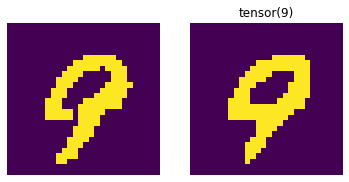
Below the original digit is on the left and the regenerated one is on the right. You can see the model is encoding and decoding the digit pretty well.
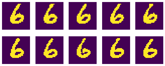
Generate more training images
We can use the generative feature of the model to produce more training images. Below is an example codes of generating more images with digit 6.
digit = 6
numSamples = 10
fig, axs = plt.subplots( int(numSamples/5), 5)
fig.set_figheight(4)
fig.set_figwidth(10)
z_digit_mean = z_mean[labels==digit]
z_digit_var = z_variance[labels==digit]
zz = z_digit_mean.mean(0) + torch.randn( (numSamples, z_digit_mean.shape[1]), device=device)*torch.sqrt(z_digit_var.mean(0))
for i in range(numSamples):
    img = decode.generateImage(zz[i]).reshape([28, 28])
    axs[int(i/5), int(i%5) ].imshow(img)
    axs[int(i/5), int(i%5) ].axis('off')
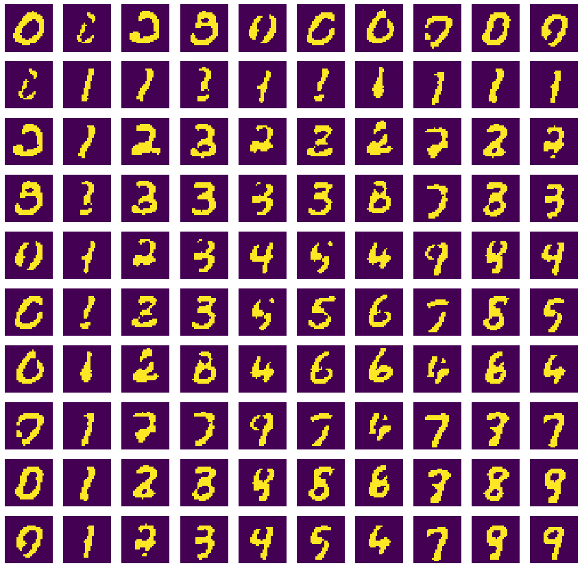
mixing digits
We can calculate the average latent variable for each digit, then average them with each other to create mixture images of two digits.
fig, axs = plt.subplots(10, 10)
fig.set_figheight(15)
fig.set_figwidth(15)
for digit1 in range(0, 10):
    for digit2 in range(0, 10):
        z1_average = z[labels == digit1].mean(0)
        z2_average = z[labels == digit2].mean(0)
        img = decode.generateImage( (z1_average + z2_average)/2).reshape([28,28])
        axs[digit1, digit2].imshow( img)
        axs[digit1, digit2].axis('off')
Interpolation
Finally, we can generate “intermediate” images between two digits through interpolation.
# interploation
digit1 = 1
digit2 = 4
fig, axs = plt.subplots(1, 10)
fig.set_figheight(1.5)
fig.set_figwidth(15)
z1_average = z[labels == digit1].mean(0).detach().cpu()
z2_average = z[labels == digit2].mean(0).detach().cpu()
from scipy.interpolate import interp1d
linfit = interp1d([0,9], np.vstack([z1_average, z2_average]), axis=0)

for i in range(10):
    z_int = torch.tensor(linfit(i))
    z_int = z_int.to(device) #.reshape([1, len(z_int)])
    z_int = z_int.float()
    img = decode.generateImage(z_int ).reshape([28,28])
    axs[i].imshow( img)
    axs[i].axis('off')
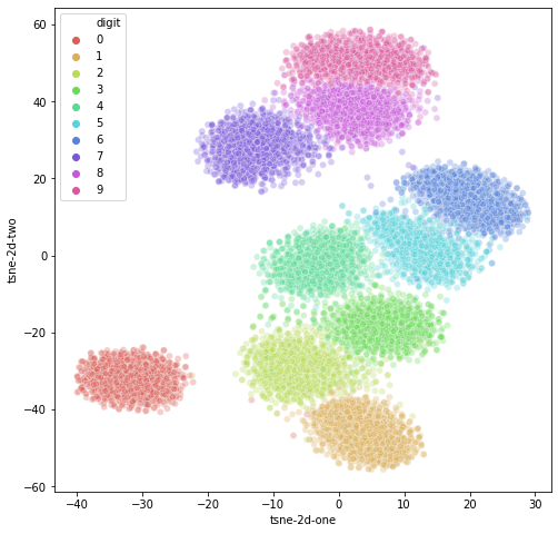
Visualize latent variables
Finally, we can visualize the high dimensional latent variables using t-SNE.
from sklearn.manifold import TSNE
import seaborn as sns
import pandas as pd
feat_cols = [ 'z'+str(i) for i in range(z.shape[1]) ]
df = pd.DataFrame(np.array(z.detach().cpu()) ,columns=feat_cols)
df['digit'] = labels
df['label'] = df['digit'].apply(lambda i: str(i))
tsne = TSNE(n_components=2, verbose=0, perplexity=40, n_iter=1000)
tsne_results = tsne.fit_transform(df)
df['tsne-2d-one'] = tsne_results[:,0]
df['tsne-2d-two'] = tsne_results[:,1]
plt.figure(figsize=(16,10))
sns.scatterplot(
    x="tsne-2d-one", y="tsne-2d-two",
    hue="digit",
    palette=sns.color_palette("hls", 10),
    data=df,
    legend="full",
    alpha=0.3
)